Learning about probability distributions can be intimidating. So many new terms and concepts. I’ll use everyday language and relatable examples.

There are many types of probability distributions. We’ll examine these three:

• Discrete Uniform Distribution: rolling a single six sided die
• Discrete Triangular Distribution: summing the face value of two dice
• Normal Distribution: height of a sample of people

Each distribution name is technical and mysterious but I’ll explain carefully 🙂

Discrete Uniform Distribution

We have a single six sided die.

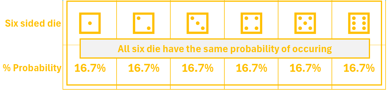
Discrete: there are a limited number of possibilities. In this case, only 6. We can never roll a 4.75 or a 2.5.

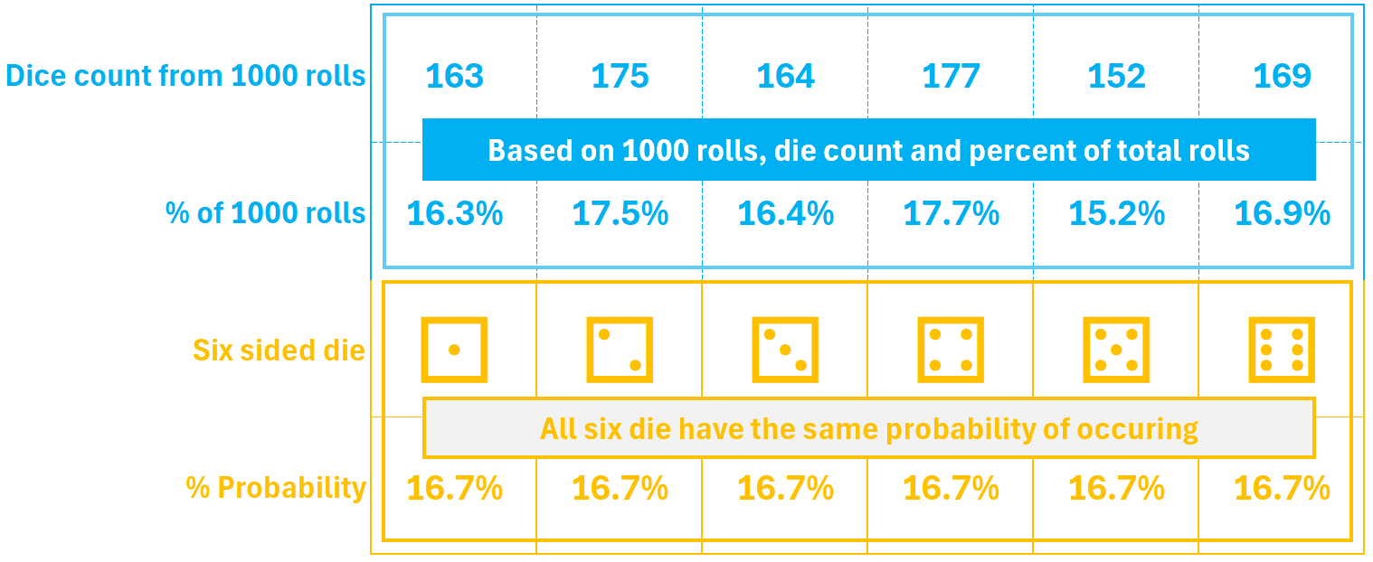
Uniform: each number has an equal 1 out of 6 possibility of being rolled (approximately 16.7%).

Anything can happen if we only roll the die 10 times but if we roll it 1000 times the percent of each roll will be very close to the 1/6 or 16.7% probability:

In theory, the more times we roll the die, the closer we’ll get to the expected uniform (even or straight) distribution. A graph helps us see that there’s no curve to sharp spike in the middle, just an almost straight horizontal line.

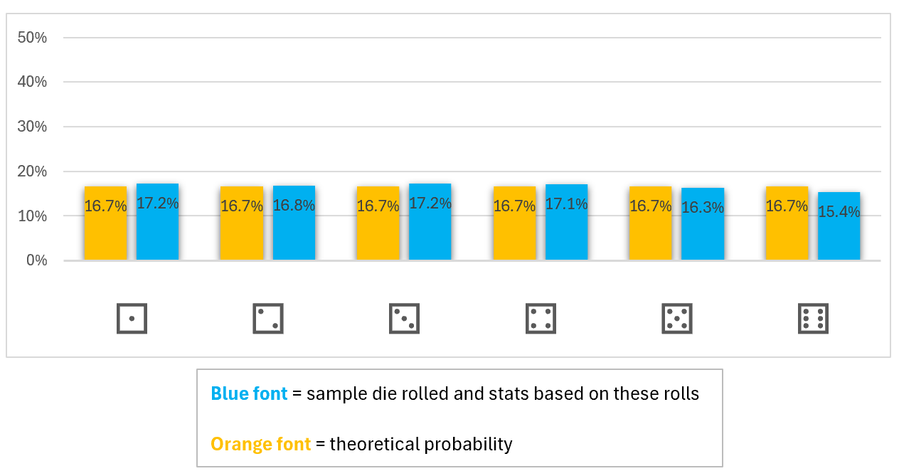
Note: I didn’t use a line or area chart as that might imply that an outcome could occur anywhere along the line or anywhere within the area. This is not possible with discrete distributions.

Discrete Triangular Distribution

I’ll use the example of rolling two six sided die and summing their face value.

Discrete: There are only 36 possible dice pairs. Each pair has the same possibility of occurring: 1/36 or approximately 2.78%.

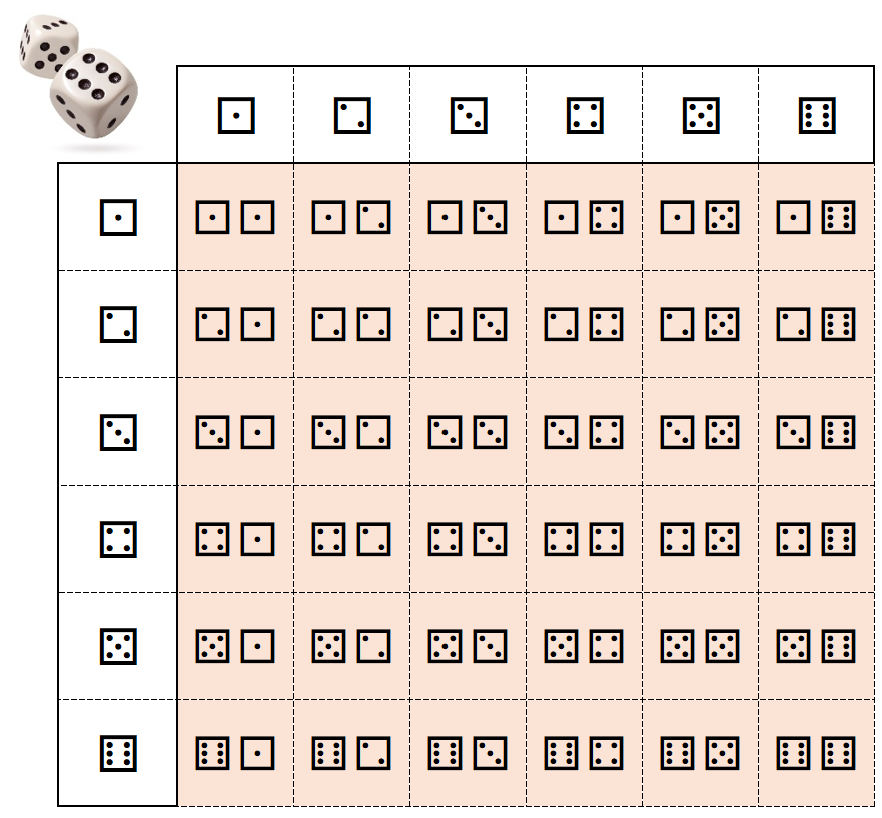
The difference is when we sum the face value of the two die. Below, the same dice pairs rearranged based on their combined sum. There are 6 different dice pairs that sum to 7.

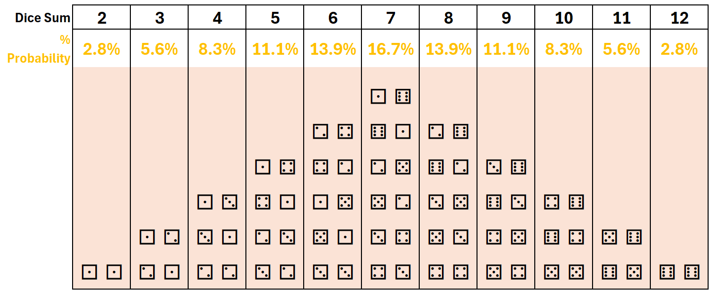
Triangular: when the dice pairs of the same sum are stacked, they resemble a triangle.

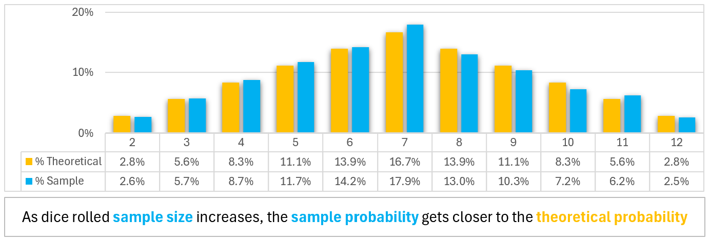
Below, the results of 1000 dice pairs (blue) closely resemble the theoretical possibilities (orange). Note the symmetry moving away, left and right, from the sum of 7 in the center.

• 7 has a 16.7% probability of occurring
• 6 and 8 have a 13.9% probability of occurring
• 5 and 9 have a 11.1% probability of occurring
• 4 and 10 have a 8.3% probability of occurring
• 3 and 11 have a 5.6% probability of occurring
• 2 and 12 have a 2.8% probability of occurring

Normal Distribution

(Read below or read this post)

We’ll use our height as an example. When we discuss height, we say things like this:

• most people are close to the average height
• some are a bit taller or a bit shorter
• in rare cases, some are very tall or very short

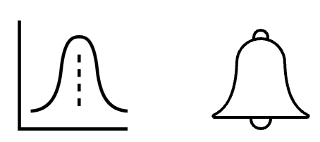
Bell Curve: these comments describe data that clusters around the average height (dotted line in graph below) with fewer data points (short and tall people) trailing off to the left and right. The chart resembled a bell and became known as normal distribution bell curve.

In keeping with the previous distribution names, a normal distribution should be referred to as a continuous normal distribution.

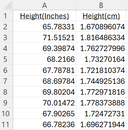
Continuous: Unlike discrete dice rolls, height can occur anywhere along a continuous range. One person can be 5 feet 10.2 inches tall (178.308 cm) and another person can be slightly taller at 5 feet 10.201 inches tall (178.31054 cm). We can’t possibly count all the possible heights of humans.

Height is often rounded down to the closest inch (or centimeter) for practical purposes. This may trick us into thinking that height is a discrete measurement but it isn’t, It’s a continuous measurement.

Symmetry: left and right sides of the curve are the same or are at least very similar.

Standard Deviation: measures how close the majority of values are from the mean (average). A larger standard deviation indicates that values are spread out more (flatter looking bell curve) while a smaller standard deviation indicates that values cluster closer to the mean.

Dataset: sample height (and weight) data from Kaggle.com. I’ll use just height data. Note how precise the height measurements are:

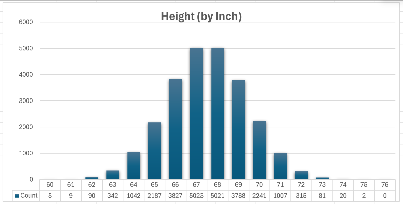
There are 25000 rows of data. This chart counts height per inch:

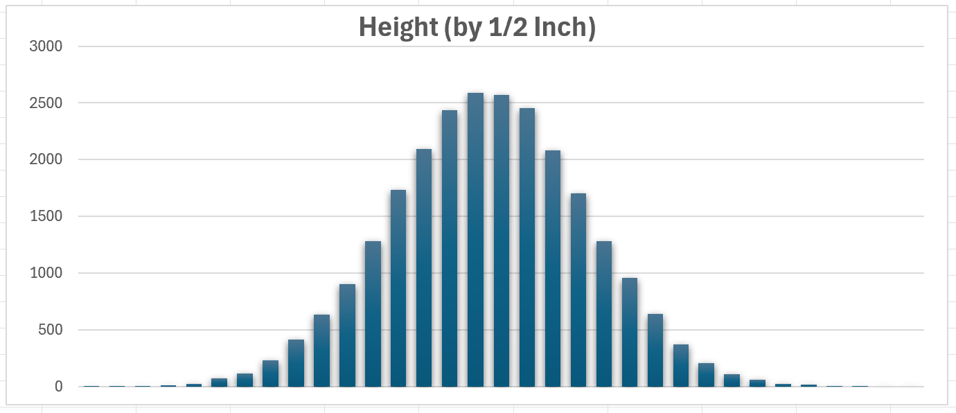
This chart counts height by 1/2 inch. The data doesn’t display well so I removed it, but we can see the smooth bell curve easier as there are more groups (columns):

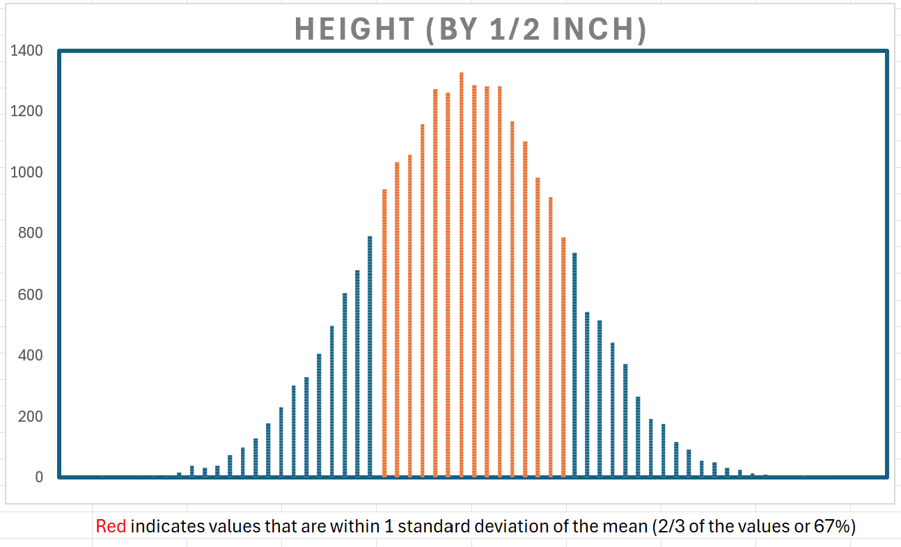
Below, values in red are those within 1 standard deviation of the mean (2/3 or 67% of the values). It helps to reinforce the idea that most people are close to the average height.

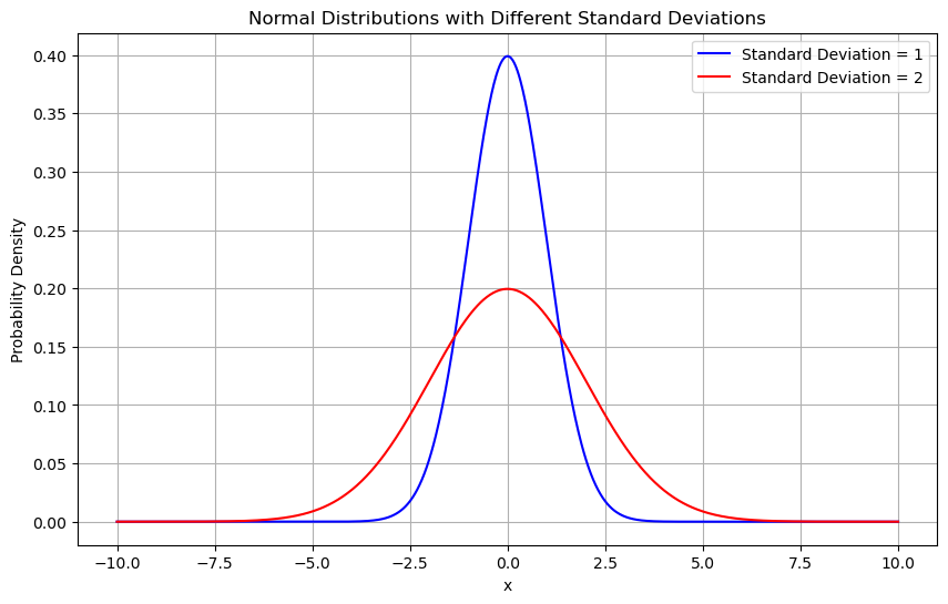
I’ve been playing around with Copilot and other AI. I asked Copilot this question: Create 2 different normal distribution graphs with different standard deviation values

Copilot’s answer: Here’s a graph comparing two normal distributions with the same mean (0) but different standard deviations

• Blue curve: Standard deviation = 1 (narrower and taller)
• Red curve: Standard deviation = 2 (wider and shorter)

This illustrates how increasing the standard deviation spreads the distribution out and lowers its peak.

Normal distribution is obviously the most complex of the three probability distributions reviewed in this post but it’s my favorite. One could dedicate their life to studying probability distributions but it’s possible for the rest of us to understand the concepts if we work at it.

Excel File

I had fun creating the Excel file.

The Excel file has four sheets:

• discrete uniform distribution: enter number of dice to be used in stats & graph
• discrete triangular distribution: enter number of dice pairs to be used in stats & graph
• continuous normal distribution: a sample of 25000 people’s height to show bell curve affect
• stats: hidden sheet with stats & graph used for linked pictures

This is my favorite formula:

=CHOOSE(RANDBETWEEN(SEQUENCE(A2,1,1,0),6), "⚀", "⚁", "⚂", "⚃", "⚄", "⚅")

It creates a column of random dice. The number of dice depends on the input value in cell A2:

Note: although the file doesn’t have as many formulas as some large models, it’s slow to calculate due to the volatile RANDBETWEEN function. A volatile function (also TODAY, NOW, etc.) is constantly recalculating. Some try to minimize/remove volatile functions at all costs…but at times we need them.

About Me

My name is Kevin Lehrbass. I’m a data analyst.

Curiosity and necessity has kept me learning for many years now. I also have to keep up with all the changes in Excel. So many new features and functions. These days I’m fascinated with Excel formulas that spill!