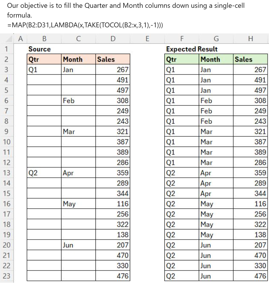
Excel BI has some fun challenges. This one has several solutions but would the average Excel user understand them?
Read more: How Does This Formula Work?AI Formula Help
These solutions were created by advanced Excel users, but more and more, people will use AI to write formulas instead of asking a professional for help. So…
How will beginning and intermediate Excel users know if their AI created formula is correct?
I’m not saying it’s AI’s fault. AI does amazing things but if the question isn’t phrased properly the solution won’t be correct. And, AI does make mistakes. Now back to Excel BI’s challenge.
Back to the Challenge
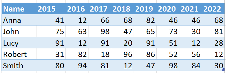
Note: I replaced original letters in columns B & E with real class subjects.
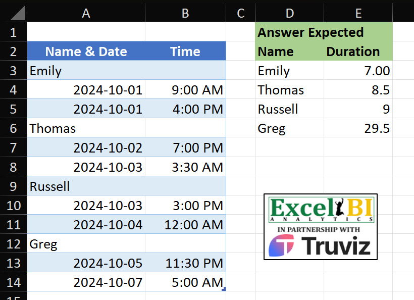
Challenge: a student takes a subject (column B) and receives a mark (column C). That mark is compared to the passing mark (column F) to determine a pass or fail grade.
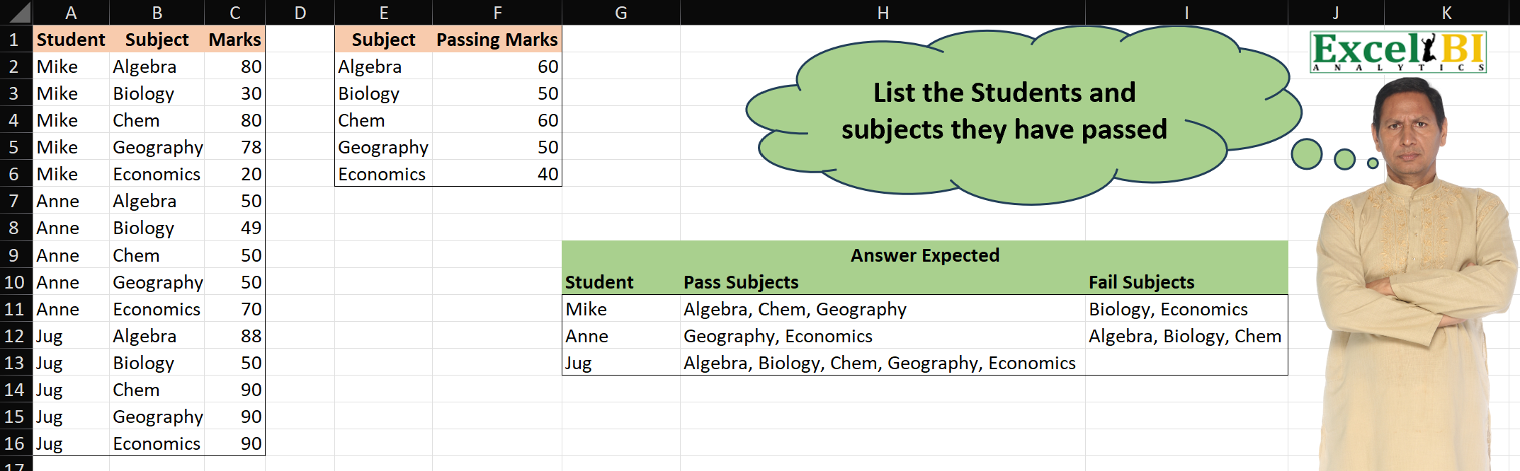
With such a small set of data, we can compare Marks with Passing Marks and easily confirm all answers:
- Mike passed Algebra, Chem, and Geography but failed Biology and Economics
- Anne passed Geography and Economics but failed Algebra, Biology, Chem
- Jug passed all subjects
Real world data sets can have 10000s of rows. We have to be sure that the formula is correct as we can’t manually check every row.
Pick a Solution!
In selecting a solution, think of this:
Could you explain the solution to a basic/intermediate user when handing off the model to them?
I realize that this doesn’t always happen, but it should!
Review the solutions in the Linkedin post comments.
My Favorite Solution
Below, the solution I like. There’s a tricky part but it’s shorter than most (all?) solutions.
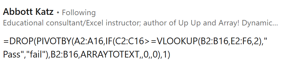
I reformatted Abbott’s formula to make it easier to read:
=DROP(
      PIVOTBY(
              A2:A16,
              IF(C2:C16>=VLOOKUP(B2:B16,E2:F6,2)," Pass","fail"),
              B2:B16,
              ARRAYTOTEXT,,0,,0
      ),
      1
 )
Abbott’s Solution Explained
Let’s start by focusing only on function PIVOTBY:
=PIVOTBY(
         A2:A16,
         IF(C2:C16>=VLOOKUP(B2:B16,E2:F6,2)," Pass","fail"),
         B2:B16,
         ARRAYTOTEXT,,0,,0
 )
Let’s examine PIVOTBY function arguments:
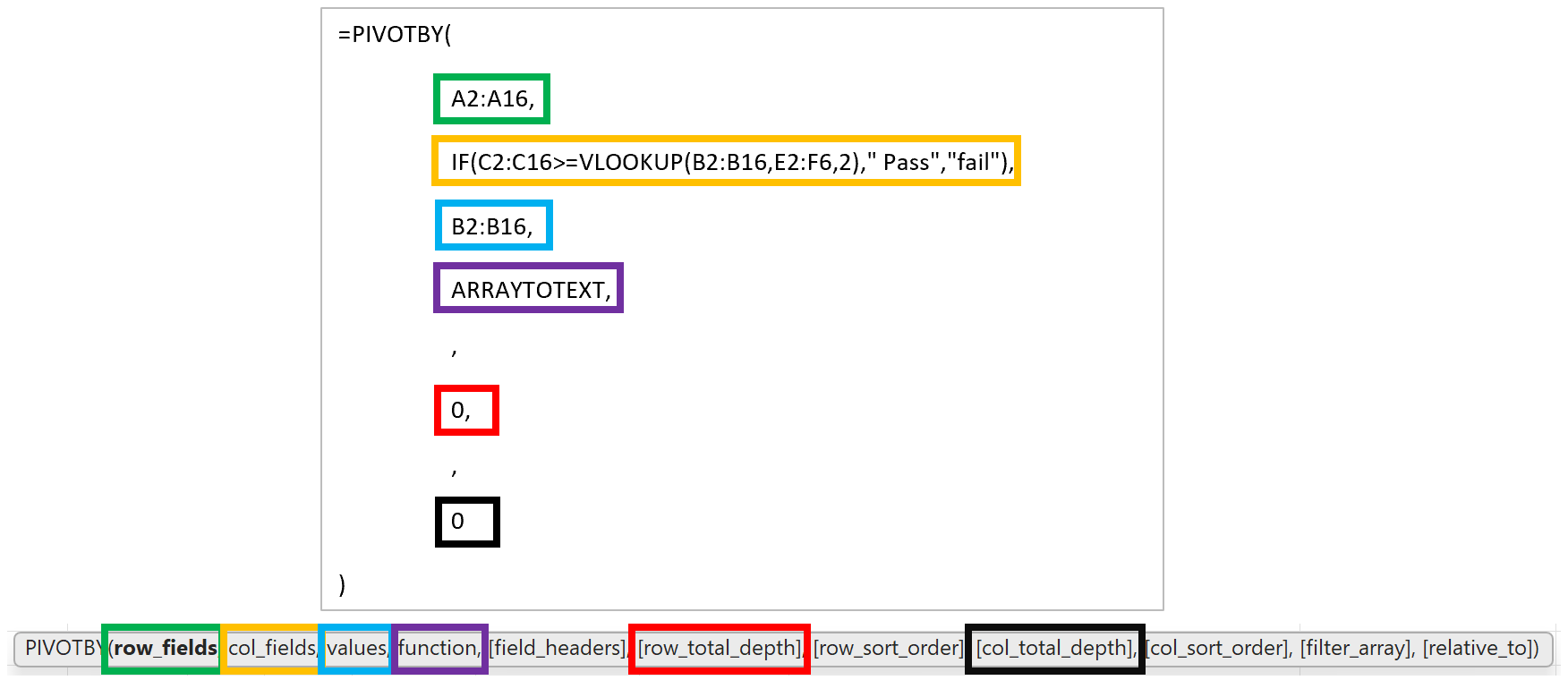
- row_fields: unique text values (students) from A2:A16
- Mike
- Anne
- Jug
- col_fields: the tricky and brilliant part!
- IF(C2:C16>=VLOOKUP(B2:B16,E2:F6,2),” Pass”,”fail”)
- normally, unique text values are spread horizontally across the top of a pivot. In this case, IF function compares all marks with their passing mark number and assigns each one to belong on the left column (” Pass”) or right column (“fail”)
- values: B2:B16 values. Not numbers to sum or average but text values!
- function: ARRAYTOTEXT aggregates (concatenates) text in a single cell
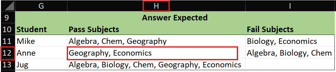
- cell H12: ‘Pass Subjects’ Geography and Economics for Anne
- other function arguments are skipped or have a value of 0
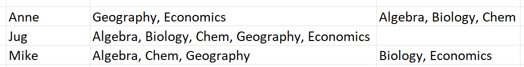
For each unique column A Student, column B Subjects are concatenated together into column ” Pass” or column “Fail” based on Mark status.
DROP function removes the top row that has text ” Pass” or “Fail”.
One thing I couldn’t initially figure out:
Why does column ” Pass” start with a space?
Pass column needs to be displayed on the left but the F in Fail comes before the P in Pass so a space is included to force Pass to the left!
Include Pivot Column Headers
Let’s add column headers to make the solution look exactly like this:
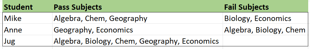
Here’s the formula:
=LET(
col_h, {"Student", "Pass Subjects", "Fail Subjects"},
formula,
       DROP(
            PIVOTBY(
                    A2:A16,
                    IF(C2:C16>=VLOOKUP(B2:B16,E2:F6,2)," Pass","fail"),
                    B2:B16,
                    ARRAYTOTEXT,,0,,0
            ),
       1
       ),
final, VSTACK(col_h,formula),
final)
LET function allows us to break logic down into steps via variables:
- col_h the three text values in the array constant are the column headers
- formula the formula that we reviewed in this post
- final VSTACK stacks variable col_h on top of formula result
About Me

My name is Kevin Lehrbass. I’m a long term Microsoft Excel user and fan. I love it! Even though I’ve worked with SQL, Power BI, etc., Excel is still my favorite. It’s everywhere and Microsoft keeps adding features and functions. I can’t wait to see what they do next!