


I’ve seen some amazing videos showcasing the potential of dynamic array functions but seeing them used in a model is even more impressive!
Advanced Excel for Financial Planning and Analysis (FP&A)
I completed Carl Seidman’s course recently. It was amazing! During the course I kept thinking:
“Dynamic array functions will definitely change how we model in Excel!“

I highly recommend this course. Learn from the videos and audit the Excel files! Even if you’re not a FP&A Excel modeler, you can learn techniques to use in your specific industry.
Carl has kindly given me permission to review one of the Excel files to show you how powerful dynamic arrays can be in building Excel models.
Workbook Sheets
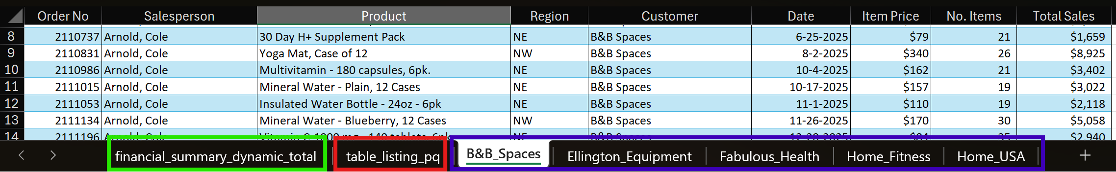
- B&B_Spaces and the four sheets to the right each have a table (one is selected as source data)
- table_listing_pq Power Query exports a list of all workbook tables (used to select source table)
- Financial_Summary_Dynamic_Total calculates using data from selected table
I hide some sheets that show other methods to summarize the data. Financial_Summary_Dynamic_Tool is Carl’s most automated solution that uses dynamic arrays.
Financial_Summary_Dynamic_Total
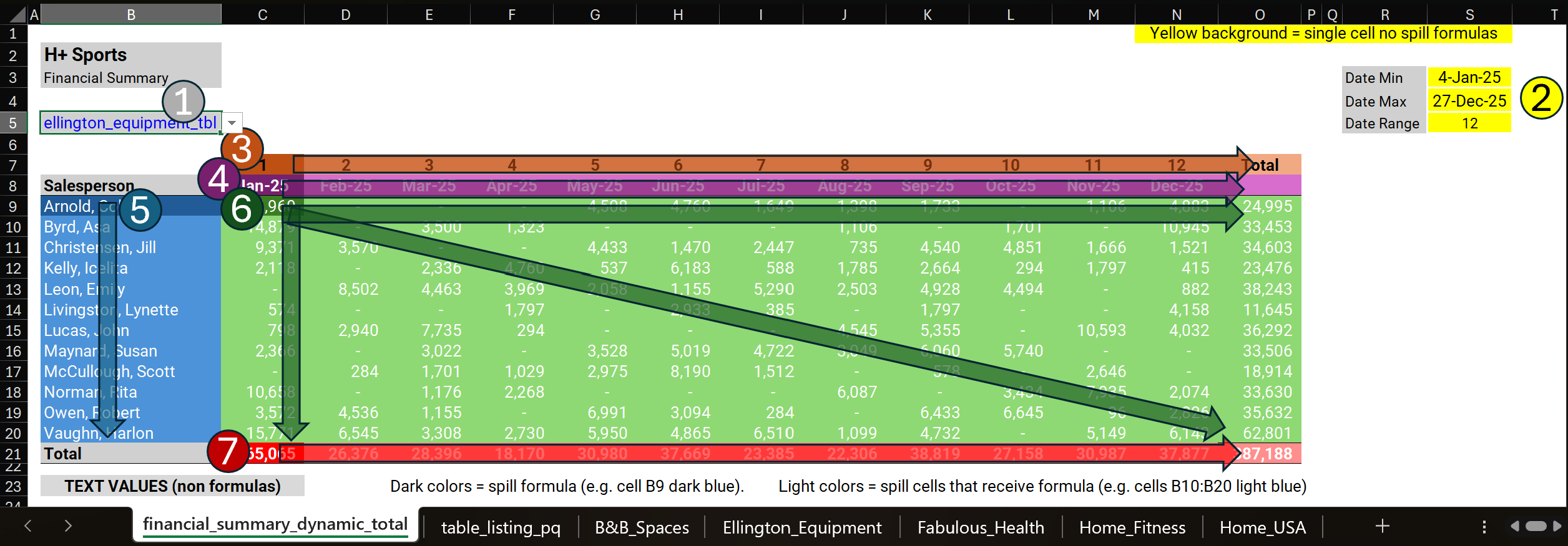
Below, sheet financial_summary_dynamic_total (click to expand picture).
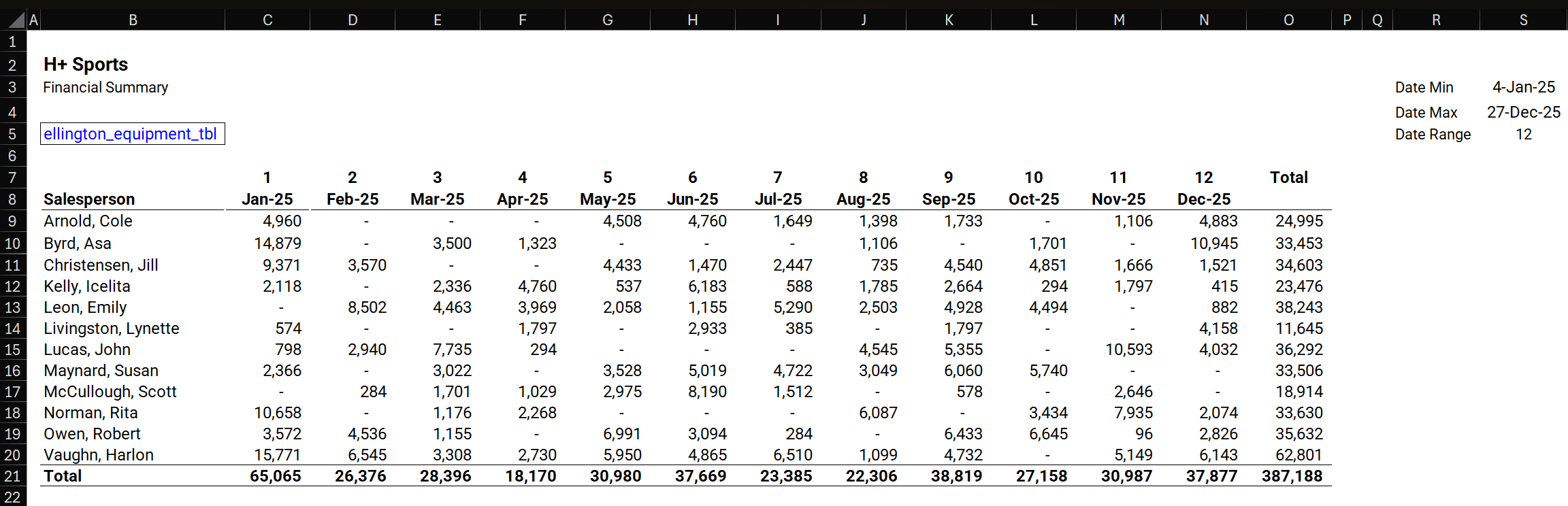
Looks simple BUT we need to consider these requirements:
- aggregate data from the table selected in cell B5 without using INDIRECT (volatile function that slows down calculations)
- aggregation calculates based on: selected table, Salesperson and Month/Year
- no manual inserting new columns and rows to accommodate extra months and salespeople
- each table may have different Salespeople and date ranges
OK, a little more complex, but still possible with a big bunch of formulas.
How many formulas do you think Carl used in this sheet?
- 150?
- 100?
- 50?
There are only 8 formulas in this sheet! (highlighted in green)
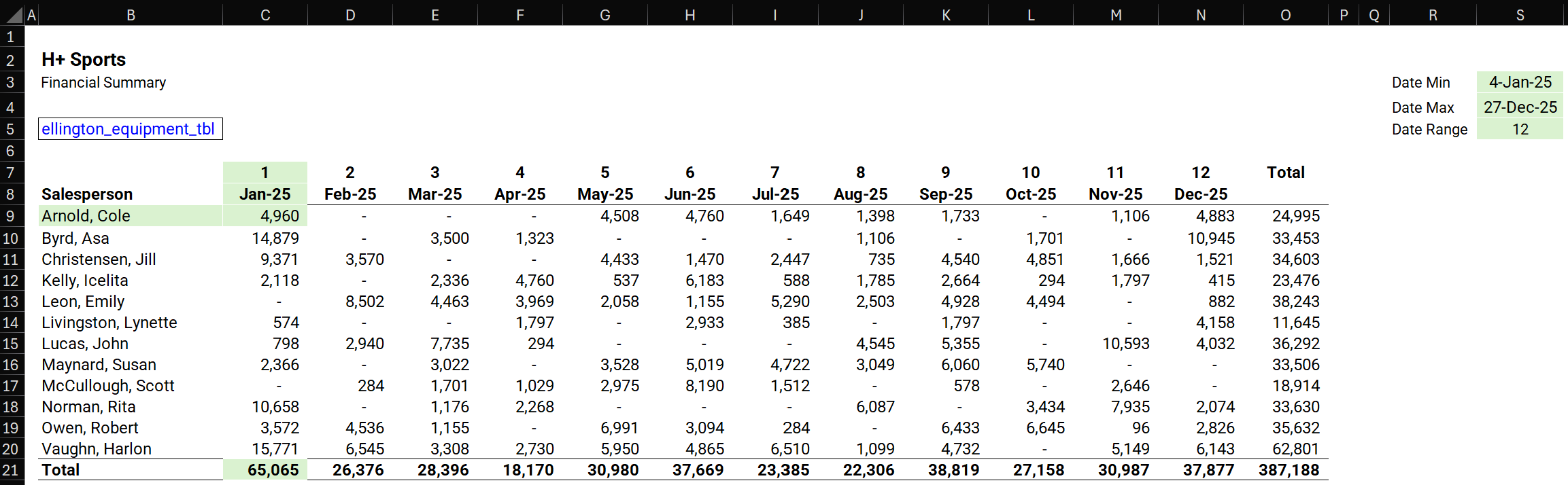
Below, dark cell formulas spill into lighter colored cells. Most dynamic arrays spill right or down but cell C9 spills right AND down! Column S formulas do not spill.
Sheet summary: 1 data validation cell, 5 formulas spill and 3 do not.
- Cell B5 select a table (sheets ‘B&B_Spaces’ to ‘Home_USA’ each have a table)
- Cells S3, S4, S5 (don’t spill) calculate min & max dates and number of months
- Cell C7 month number sequence spills right and ends with word ‘Total’
- Cell C8 calculate and spill dates to the right
- Cell B9 create unique salesperson list from selected table (cell B5)
- Cell C9 SUMIFS on Total Sales column based on table name, salesperson, date
- Cell C21 total row sums the values above in each column
And now the formulas!
3 Non Spill Formulas
Cell S3
Minimum [Date] column value based on selected table:
=MIN(
SWITCH($B$5,
table_listing_pq!$B2,bb_spaces_tbl[Date],
table_listing_pq!$B3,ellington_equipment_tbl[Date],
table_listing_pq!$B4,fabulous_health_tbl[Date],
table_listing_pq!$B5,home_fitness_tbl[Date],
table_listing_pq!$B6,home_usa_tbl[Date]))
Cell S4
Maximum [Date] column value based on selected table:
=MAX(
SWITCH($B$5,
table_listing_pq!$B2,bb_spaces_tbl[Date],
table_listing_pq!$B3,ellington_equipment_tbl[Date],
table_listing_pq!$B4,fabulous_health_tbl[Date],
table_listing_pq!$B5,home_fitness_tbl[Date],
table_listing_pq!$B6,home_usa_tbl[Date]))
Cell S5
Calculates number of months given min & max dates from selected table:
=ROUND((S4-S3)/30,0)5 Spill Formulas
Cell C7
SEQUENCE creates a counter, EXPAND adds “Total” on the right.
=EXPAND(SEQUENCE(1,S5,1,1),,$S$5+1,"Total")Cell C8
EOMONTH normally returns a single date but SEQUENCE provides multiple values and causes the spill. EXPAND adds a space on the right.
=EXPAND(EOMONTH($S$3,SEQUENCE(1,$S$5,0,1)),,$S$5+1,"")Cell B9
Based on the table selected in cell B5, a sorted salesperson list is created.
=SORT(
UNIQUE(
SWITCH($B$5,
   table_listing_pq!$B2,bb_spaces_tbl[Salesperson],
   table_listing_pq!$B3,ellington_equipment_tbl[Salesperson],
   table_listing_pq!$B4,fabulous_health_tbl[Salesperson],
   table_listing_pq!$B5,home_fitness_tbl[Salesperson],
   table_listing_pq!$B6,home_usa_tbl[Salesperson]
)))
Cell C9
Long but logical formula. Each SUMIFS part is created separately.
XMATCH creates a number used by each “…_col” variable to retrieve selected table column values.
HSTACK inserts the Row_total after SUMIFS is finished in each row.
Salespeople_list references cell B9 spill causing this formula to spill down.
Variables start_date & end_date cause it to spill right.
=LET(selection,      XMATCH($B$5,table_listing_query[Name],0),

    sales_col,       CHOOSE(selection,
                           bb_spaces_tbl[Total Sales],
                           ellington_equipment_tbl[Total Sales],
                           fabulous_health_tbl[Total Sales],
                           home_fitness_tbl[Total Sales],
                           home_usa_tbl[Total Sales]),

    salesperson_col, CHOOSE(selection,
                          bb_spaces_tbl[Salesperson],
                          ellington_equipment_tbl[Salesperson],
                          fabulous_health_tbl[Salesperson],
                          home_fitness_tbl[Salesperson],
                          home_usa_tbl[Salesperson]),

    dates_col,       CHOOSE(selection,
                          bb_spaces_tbl[Date],
                          ellington_equipment_tbl[Date],
                          fabulous_health_tbl[Date],
                          home_fitness_tbl[Date],
                          home_usa_tbl[Date]),

    salespeople_list, $B$9#,

    start_date, ">=" & DATE(YEAR(DROP($C$8#,,-1)),
                       SEQUENCE(1, $S$5,  MONTH(DROP($C$8#,,-1))), 1),

    end_date,   "<=" & DROP($C$8#,,-1),

    result, SUMIFS(sales_col, salesperson_col, salespeople_list, dates_col,
                   start_date, dates_col, end_date),

    row_total, BYROW(result,SUM),

    HSTACK(result,row_total)
)
Yes, cell C9 formula requires time to audit but it’s the only long formula in the workbook. All other formulas are short and simple. I’d rather audit a single long formula versus dozens of messy formulas.
C21
BYCOL function looks at cell C9 spill and sums above per column as far right as needed.
=BYCOL(C9#,SUM)Sheet table_listing_pq
Carl created a simple query, that’s exported to sheet table_listing_pq, to list all workbook tables. Below, we see the Power Query M code.
let
    Source = Excel.CurrentWorkbook(),
    #"Filtered Rows" = Table.SelectRows(Source, each Text.EndsWith([Name], "tbl"))
in
    #"Filtered Rows"
This is used by XMATCH and CHOOSE functions in sheet financial_summary_dynamic_total (cell C9).
Auditing Models
I have created and audited Excel models for almost 25 years. Many are disasters and require dozens of hours to audit, and redevelop.
Carl’s model was easy to audit. There’s only one long formula but I wouldn’t even call it a complex formula. It reminds me of T-SQL: build all the pieces, test from carefully, then put them together.
Another Reason to Learn Dynamic Arrays
When dynamic arrays were initially introduced a few years ago, backwards compatibility was a major concern. Companies not using Excel 365 version couldn’t use models built with dynamic arrays.
Fast forward to the present…more and more (most?) companies use Excel 365 so learning how to audit and use dynamic arrays has become a necessity. Don’t be left behind!
Simplicity
On the other hand…I’ve seen cases in which dynamic arrays were not necessary. I’ve seen very complicated formulas that are almost impossible to decipher. Remember to be kind to those who will be using the models you create.
Another reason why I really enjoyed Carl’s course: he utilized the power of dynamic array functions without making them overly complicated. Powerful and logical formulas! The right mix.
About Carl Seidman

Carl Seidman is a renowned business advisor and educator specializing in financial planning and analysis (FP&A), business strategy, and finance transformation. He has coached thousands of finance professionals across Fortune 500 companies and middle-market firms, helping them build sustainable models and elevate their careers. As a Microsoft MVP and Certified Speaking Professional, Carl combines technical expertise with engaging communication, making complex financial concepts accessible. He holds degrees in finance, economics, and accounting from Michigan State University and teaches data analytics as an adjunct professor at Rice University.
https://seidmanfinancial.com/
https://www.linkedin.com/in/carlseidman
About Me

My name is Kevin Lehrbass. I’m a Data Analyst and I live in Milton, Ontario, Canada. Fenton and Cali are my amazing dogs!
Microsoft Excel is my favorite software and the last few years have been incredible as more and more new functions and features have been introduced. I’ve been learning about dynamic array functions and I really enjoyed and learned a lot from Carl’s course.
Pingback: Segmenting Data in Microsoft Excel | My Spreadsheet Lab