Create a solution we can understand

Recently, a client asked me to create an Excel model that they could fully understand and modify if needed. That comment changed my thought process on how to solve it.

Read more: Create a solution we can understand

Audit friendly model

There are different types of Excel models. In some cases, the logic is very complex and there’s no easy way to solve it. It may not be possible to explain everything to end users who have basic skills. End users use the model and never understand how the formulas / code works.

However, sometimes a client has strong Excel knowledge and requests a model that can be understood and modified in places. It may be possible to accommodate this request if the model is built carefully.

What does strong Excel mean?

There are endless ways to assess Excel knowledge. I like the hierarchy from Financial Modeling World Cup.
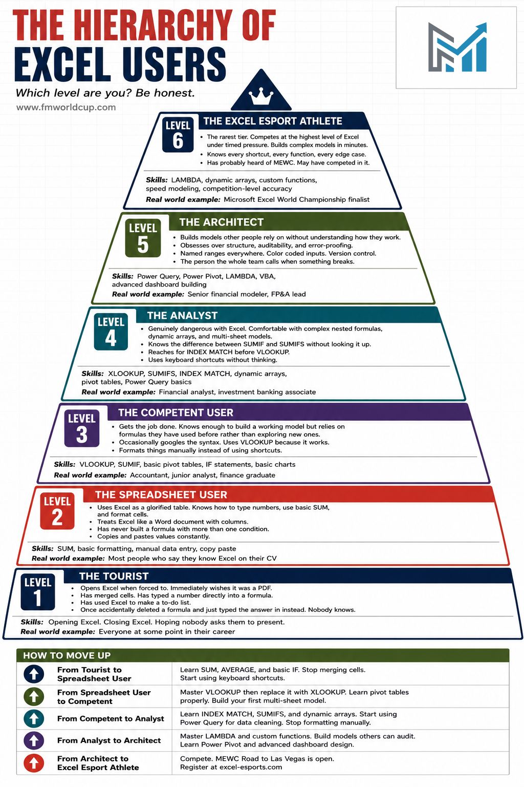
My client’s Excel skills are mostly level 3. I believe my Excel skills are mostly level 5. More on this hierarchy later.

How did I build the model?

I broke down the logic into smaller components. This may not always be possible but it was in this case.

I limited my use of dynamic array functions: one UNIQUE and one FILTER. Why? Dynamic array functions can perform magic but most are too complex for the average user especially when several are nested in the same formula. Here’s a list of dynamic array functions from www.ablebits.com

  • UNIQUE extracts unique items from a range of cells.
  • FILTER filters data based in the criteria you define.
  • SORT sorts a range of cells by a specified column.
  • SORTBY sorts a range of cells by another range or array.
  • RANDARRAY generates an array of random numbers.
  • SEQUENCE generates a list of sequential numbers.
  • TEXTSPLIT splits strings by a specified delimiter across columns or/and rows.
  • TOCOL converts an array or range to a single column.
  • TOROW transform a range or array into a single row.
  • WRAPCOLS converts a row or column into a 2D array based on the specified number of values per row.
  • WRAPROWS re-shapes a row or column into a 2D array based on the specified number of values per column.
  • TAKE extracts a specified number of contiguous rows or columns from the start or end of an array.
  • DROP removes a certain number of rows or columns from an array.
  • EXPAND grows an array to the specified number of rows and columns.
  • CHOOSECOLS returns the specified columns from an array.
  • CHOOSEROWS extracts the specified rows from an array.
  • GROUPBY groups and aggregate data in rows based on the values in one or more columns.
  • PIVOTBY groups data in rows and columns and aggregate the values.
  • BYROW applies a specified function to each row in a range and returns one result per row.
  • BYCOL performs a specified calculation on each column in a given range.
  • TRIMRANGE removes blank columns and/or rows a range’s outer edges.
  • MAP performs a custom calculation on each value in an array.
  • SCAN processes an array of values sequentially and returns every intermediate result.
  • REDUCE iterates through an array and returns one final aggregated value.

I can’t share the solution I created for my client but I found an Excel BI challenge that I’ll use to demonstrate the idea.

Excel BI challenge

Excel BI has dozens of fun Excel challenges! Visit their ExcelBI website! This challenge asks us to rearrange column A data into rows and columns as seen below in columns C to H:
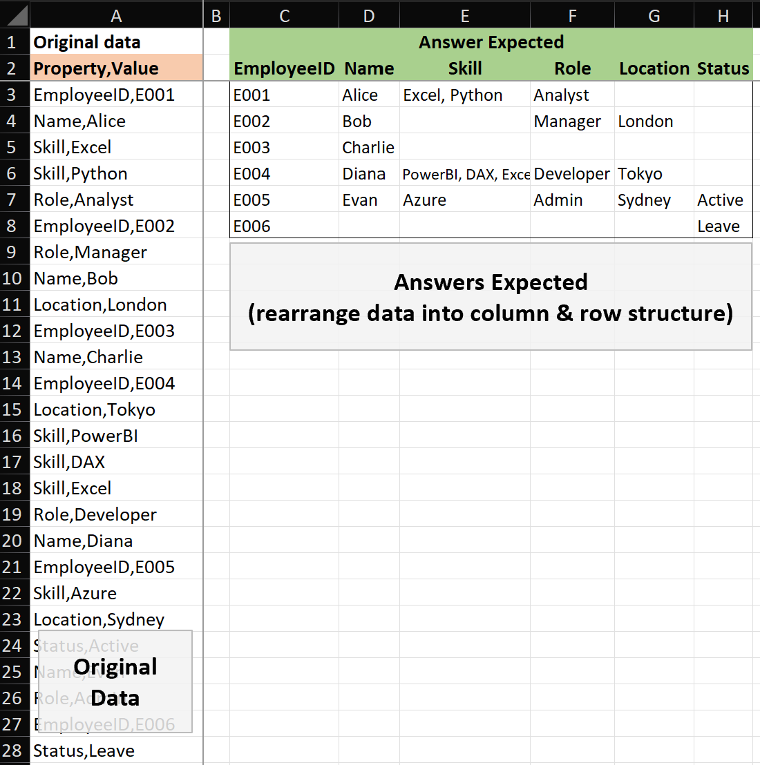
Examine the data!

It’s ESSENTIAL to carefully examine the data and the requirements.
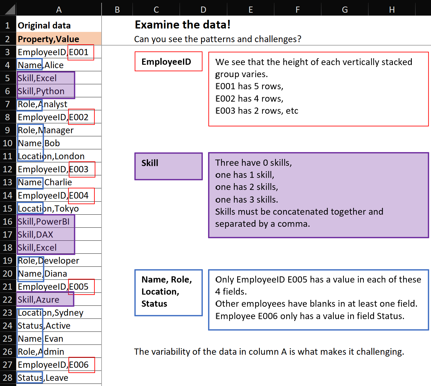
The challenge: each EmployeeID group is different as explained in the picture above. To start, we can separate the groups using the EmployeeID code highlighted in red.

Complex single cell formulas

Solutions using single cell formulas with multiple dynamic array functions. Each formula comes from a comment posted on Excel BI’s LinkedIn challenge post.

If you understand these formulas then you are a level 5 or 6 Excel user! If you can read them, like you read a sentence in the newspaper, then you might be Diarmuid Early!

=LET(i,A3:A28,j,GROUPBY(SCAN(,REGEXEXTRACT(i,"E\d+|$"),LAMBDA(x,y,IF(y="",x,y))),i&";",CONCAT,,0),HSTACK(TAKE(j,,1),REGEXREPLACE(TAKE(j,,-1),"((?<="&{"Name","Skill","Role","Location","Status"}&",)([^;]+))(?=.*((?1)))?|.","$2${3:+, }")))
=LET(s,A3:A28,k,TEXTBEFORE(s,","),v,TEXTAFTER(s,","),g,SCAN(0,k,LAMBDA(a,b,a+(b="EmployeeID"))),u,UNIQUE(FILTER(g,g>0)),uu,TOROW(UNIQUE(k)),DROP(REDUCE("",u,LAMBDA(x,id,VSTACK(x,MAP(uu,LAMBDA(h,LET(z,FILTER(v,(g=id)*(k=h),""),IF(h="Skill",TEXTJOIN(", ",,z),IFERROR(TAKE(z,-1),"")))))))),1))
=LET(a,A3:A28,b,TEXTSPLIT(a,","),c,TEXTAFTER(a,","),d,XMATCH(b,b),e,SCAN(0,d=1,SUM),DROP(PIVOTBY(e,HSTACK(d,b),c,ARRAYTOTEXT,,0,,0,,,3),1,1))
=LET(i,DROP(TEXTSPLIT(CONCAT("/"&A3:A28),{",","ID"},"/",,,""),1),g,SCAN(0,TAKE(i,,-1),LAMBDA(a,b,IF(b="",a,b))),u,TAKE(i,,1),e,DROP(PIVOTBY(g,HSTACK(MATCH(u,u,0),u),CHOOSECOLS(i,2),ARRAYTOTEXT,,0,,0),1),HSTACK(VSTACK("EmployeeID",DROP(TAKE(e,,1),1)),DROP(e,,2)))
=LET(z,A3:A28,f,LAMBDA(x,x(z,",")),a,f(TEXTBEFORE),b,UNIQUE(a),DROP(PIVOTBY(SCAN(,IFERROR(SEARCH("id",z),0),SUM),HSTACK(XLOOKUP(a,b,SEQUENCE(ROWS(b))),a),f(TEXTAFTER),ARRAYTOTEXT,,0,,0),1,1))
=LET(d,A3:A28,p,TEXTSPLIT(d,","),DROP(PIVOTBY(SCAN(0,d<"F",SUM),HSTACK(XMATCH(p,p),p),TEXTAFTER(d,","),ARRAYTOTEXT,,0,,0),1,1))

Splitting the logic into smaller bits

Excel BI’s challenge can be solved by splitting the logic into smaller pieces. To keep it simple, I also did this:

  • I only used 2 dynamic array functions: UNIQUE and FILTER
  • No mega formulas: each formula uses 3 functions or less
  • Steps are clearly labelled starting in column K
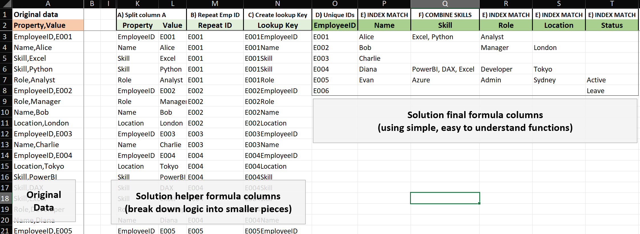
  • A) Split column A =TEXTBEFORE(A3,”,”) extracts text before the comma, =TEXTAFTER(A3,”,”) extracts text after the comma
  • B) Repeat Emp ID =IF(ISNUMBER(RIGHT(L3,1)+0),L3,M2) repeats EmpID down column M so we know where each group starts and ends
  • C) Create lookup Key =M3&K3 I could have included this key inside the final formulas but it helps to see the key in column N
  • D) Unique IDs =UNIQUE(M3:M28) creates unique list of range M3:M28 values. It’s a dynamic array function but I think it’s easy to understand. Do you agree?
  • E) INDEX MATCH =IFERROR(INDEX($L$3:$L$28,XMATCH($O3&P$2,$N$3:$N$28)),””) columns P, R, S, and T all use this formula to retrieve a single value
  • F) COMBINE SKILLS =TEXTJOIN(“, “,,FILTER($L$3:$L$28,$N$3:$N$28=$O3&Q$2,””)) a difficult formula to understand but it’s short. I could solve it without functions TEXTJOIN and FILTER, but it would need many steps and be confusing to explain

Yes, Step F COMBINE SKILLS formula might take time to explain but I think a level 3 Excel user could understand it.

=FILTER($L$3:$L$28,$N$3:$N$28=$O3&Q$2,"")

Start with the inner part of the formula above. The answers come from column L. Column N is filtered based on a key that combines column O EmployeeID with cell Q2 text “Skill”.

TEXTJOIN is wrapped around FILTER function to put all the skills together. Cell Q3 formula is dragged down the column.

=TEXTJOIN(", ",,FILTER($L$3:$L$28,$N$3:$N$28=$O3&Q$2,""))

Obviously, it would be much easier to explain all my formulas in person. I’d be able to break down each formula and also answer questions.

How many times have we heard the feedback “You’ve lost me!”. We aren’t always expected to explain the solution but when we are, it’s best to create a solution that is easier to follow/explain is smaller logical steps.

Financial Modeling World Cup

Hierarchy of Excel Users

We could debate the number of levels there should be and exactly what criteria should belong in each one for hours, but I like their hierarchy. The vast majority of Excel users are level 3 or below. The hierarchy would be much wider at the bottom and narrower towards the top but it’s not intended to be to scale.

Level 6, The Excel Esport Athlete, is an incredibly elite level of Excel and they can solve challenges incredibly fast! At the top of level 6 are only a few individuals like Diarmuid Early.

Who are they?

Learn more about them on their LinkedIn profile and their website. They have done an incredible job of turning Microsoft Excel competitions into exciting and popular events!

They organize the following events:

  • Financial Modeling World Cup
  • Excel Esports battles
  • Microsoft Excel World Championship
  • Microsoft Excel Collegiate Challenge

www.ablebits.com

I have visited ablebits website many times over the years. I like their clearly written Excel posts. They explain and demonstrate concepts very well. They have non Excel material, but my visits are all Excel 🙂

About Me

I just finished a contract. Hire me 🙂 !

I’ve worked with data for a long time and I still enjoy it! I have experience in Power BI and SQL but my strongest and favorite skill is still Microsoft Excel. I worked on an Excel hotline for 15 years and loved it 🙂
The popularity of Excel competitions has really grown over the years. I’m going to look into my local chapter here in Canada.

Learn Power Query M code

If you’re intimated by M code, this post is for you. I’ll explain techniques I use for understanding M code.

Read more: Learn Power Query M code

M code?

Power Query is a Microsoft ETL tool used in Excel and Power BI. M code is generated when we interact with the user interface to change our data.

Challenge

We need a good problem to learn from. This fun challenge is from an Excel BI Analytics LinkedIn post. Thank you Vijay A. Verma!

Requirement

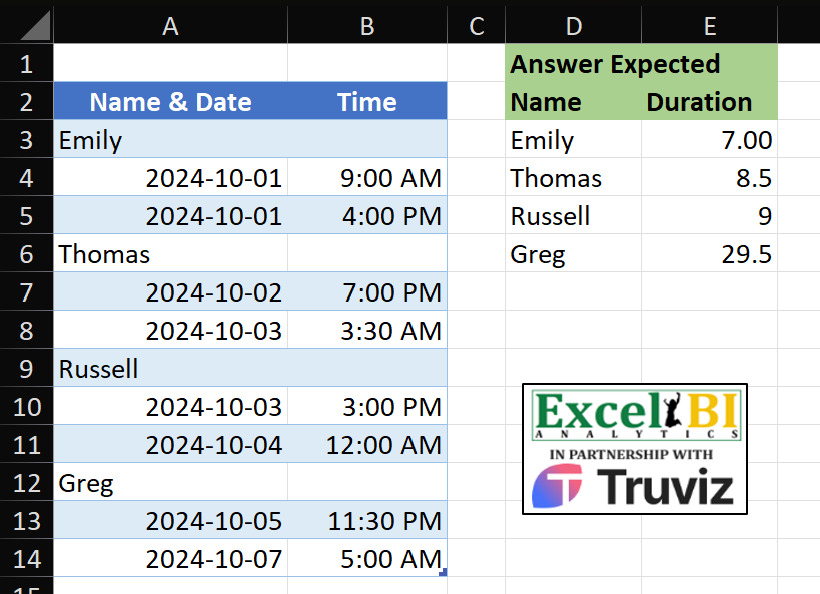
Given the data on the left, rearrange and calculate it to end up with data on the right. Each person has a start Date & Time to be subtracted from their end Date & Time to provide a time duration.

This is a sample. Imagine a real data-set with 200000 rows! Here’s the Power Query M code from Kris Jaganah that we WILL understand soon!

let
 A = Excel.CurrentWorkbook(){[Name="Table1"]}[Content],
 B = Table.ToColumns(A),
 C = List.Select( B{0}, each Text.From(_)=_),
 D = List.Transform( List.Difference( B{0}, C ),Number.From),
 E = List.Transform( List.Split( List.Transform({0..List.Count(D)-1}, each D{_} +List.RemoveNulls( B{1}){_}),2) , (x)=> (x{1}-x{0})*24),
 F = Table.FromColumns( {C,E},{"Name","Duration"})
in
 F

Why is all this M code necessary? We have bad data. Name & Date has two different data items. That shouldn’t happen! We have three items:

  • Name
  • Start Date Time
  • End Date Time.

Each should be a separate column. But Power Query & M can solve this.

Techniques to Understand M Code

When auditing a Power Query solution I do this:

  • examine raw data and think about required steps
    • what needs to be done?
    • what’s the most challenging part?
  • open Power Query, study applied steps one by one, back and forth
    • it REALLY helps to see how the data changes in every step
  • open Advanced Editor to study M code
    • compare applied steps to M code (steps are converted into M code)
    • hover over M functions to see syntax (visit documentation)
    • some steps are simple, others combine functions (write it out on paper)
    • break long steps into new queries to see data created

I assumed Kris would rearrange data to a row per person with three columns: Name, Start Date Time, End Date Time. I was wrong and learned a lot!

Examine Raw Data

There’s a million ways to solve this but all solutions will have to:

  • extract text names from Name & Date
  • add Time to Date for each row
  • per person calculate Start Date Time & End Date Time difference
  • horizontally align Name and Duration (columns D & E)

Applied Steps

Open Power Query

We don’t have to load data as we are auditing an existing solution.

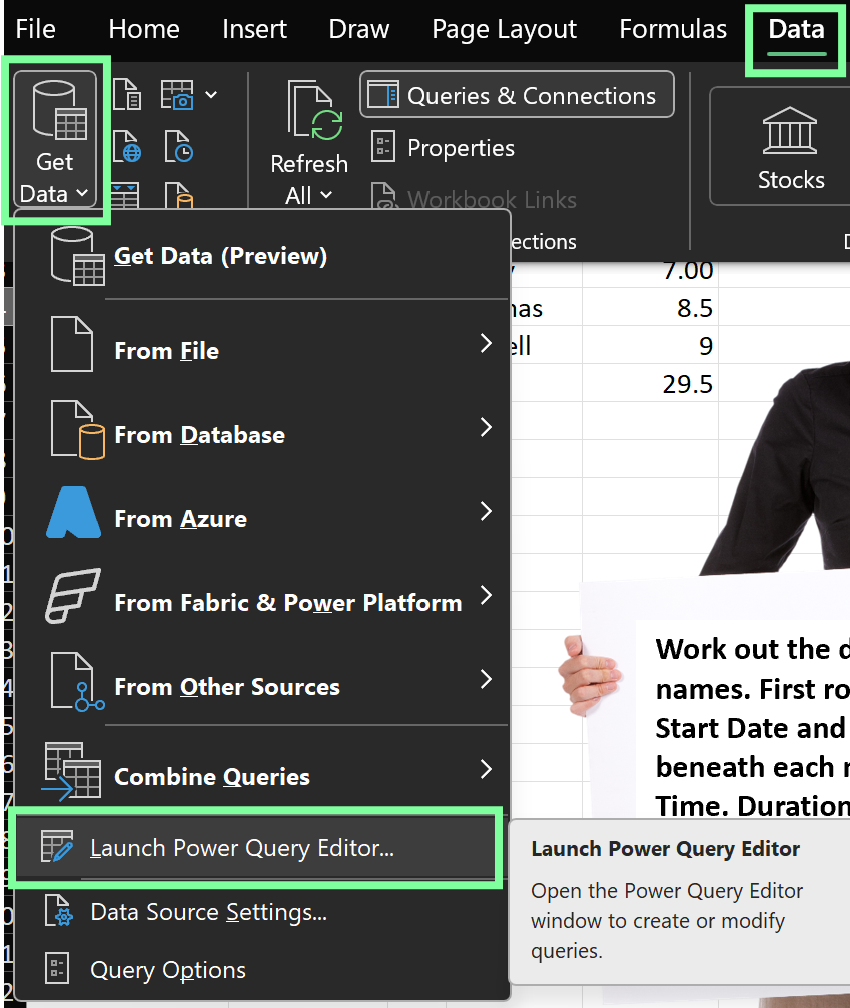
  • on the ribbon select Data
  • on the left select Get Data
  • select Launch Power Query Editor

Study Applied Steps

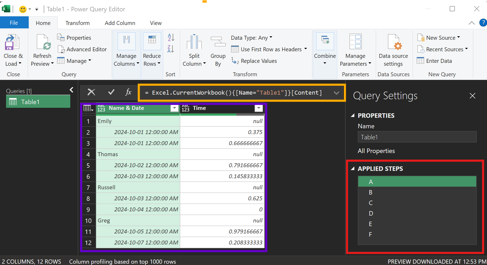
  • data preview: what the data looks like after each step
  • applied steps: examine each step to see how the data has changed
  • formula bar: formula syntax generated by each applied step

We’ll start at the beginning with step A!

Step A

Under APPLIED STEPS, click A. Formula bar shows us this code:

= Excel.CurrentWorkbook(){[Name="Table1"]}[Content]

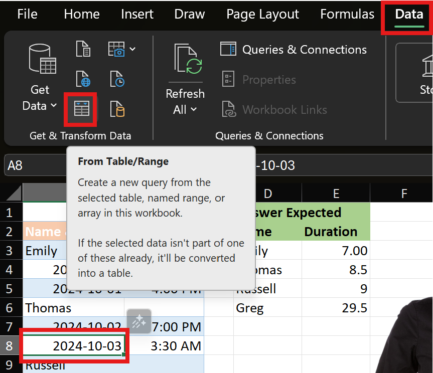
Kris loaded Table1, which we saw in sheet1, into Power Query:

  • active cell is anywhere within Table1 (cell A8 below)
  • select Data on the ribbon
  • select icon From Table/Range (section Get & Transform Data)

If you’re recreating this solution from the beginning please note:

  • by default, importing a table creates step Source. Kris renamed it to A.
  • he removed auto step Changed Type (P.Q. trying to help us…not needed here)

Excel.CurrentWorkbook imports data from the current Excel file. It belongs to a category of functions that connect to and import data.

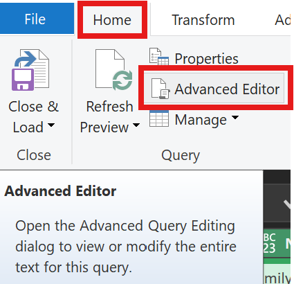
Now, we’ll look behind the curtain at the M code! On the ribbon select Home and Advanced Editor:

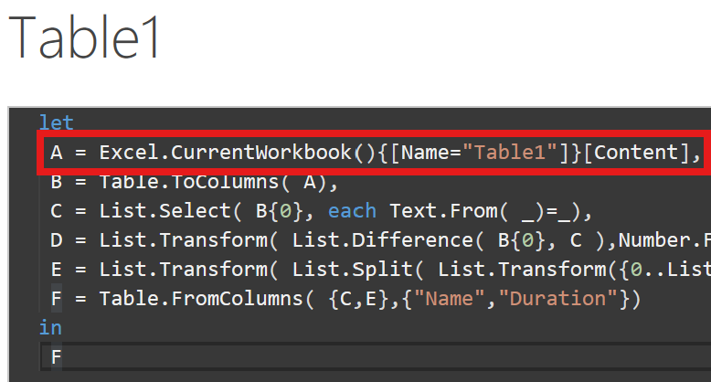
Step A has a slightly different syntax than in the formula bar. Note:

  • keyword let is before all steps
  • step name (A) is listed followed by = and the formula bar code
  • each step, except the last one, ends with a comma
  • keyword in is after all steps (unless there’s a nested let & in!)
  • our final data (answer), typically the last step (F), is after in

In the bottom right corner select Close.

Now, prepare yourself for a wild ride into the magical realms of M code!

Step B

In step B, don’t think about WHY (that’s answered in a future step). Focus on WHAT’s happening for now.

Under APPLIED STEPS, click B. Formula bar shows us this code:

B = Table.ToColumns(A),

Function Table.ToColumns references step A. Table.ToColumns syntax is:

Table.ToColumns(table as table) as list

To understand step B, we need to review Structured Types. Think of them as things: planes, trains, and cars that share a common purpose (take you somewhere) but are all unique.

Structured Types: collections of things or values:

table most common Power Query object type (step A is a table). A collection of data organized in rows and columns (like a database)

list ordered sequence of values. Lists have a single column. Step B uses list function Table.ToColumns to convert Step A columns into a list

record named fields, like a row in a table. Records represent individual data entries

Each type has it’s own functions that perform actions.

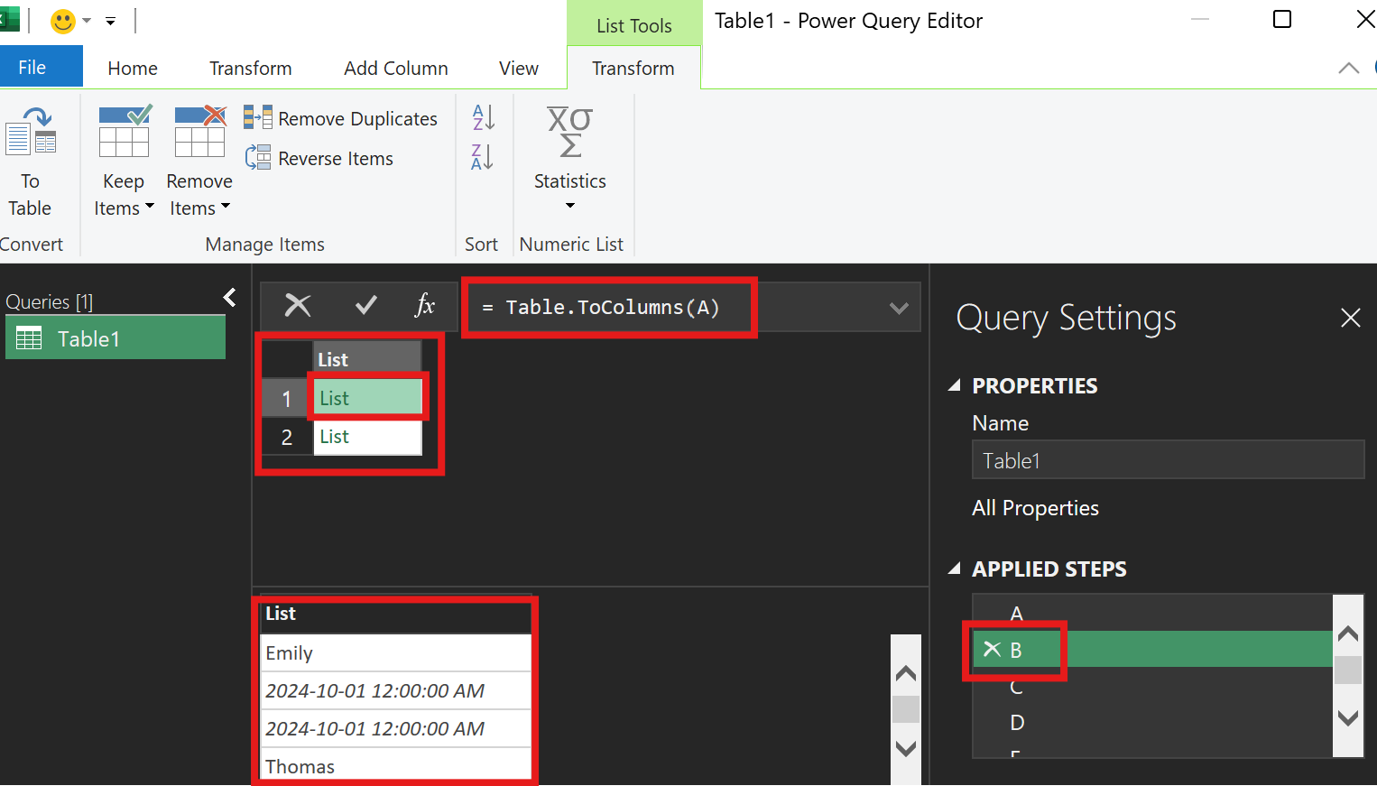
Below, in step B, note the following:

  • list function Table.ToColumns references step A table and creates a list
  • it’s a list with nested lists! Step A’s table columns have become lists in step B!
  • I selected the first nested list to peer inside: all step A column Name & Date values are inside

We’ll get to the WHY, but at least we understand WHAT happened in step B. Feel free to glance at the M code in the Advanced Editor again.

Step C

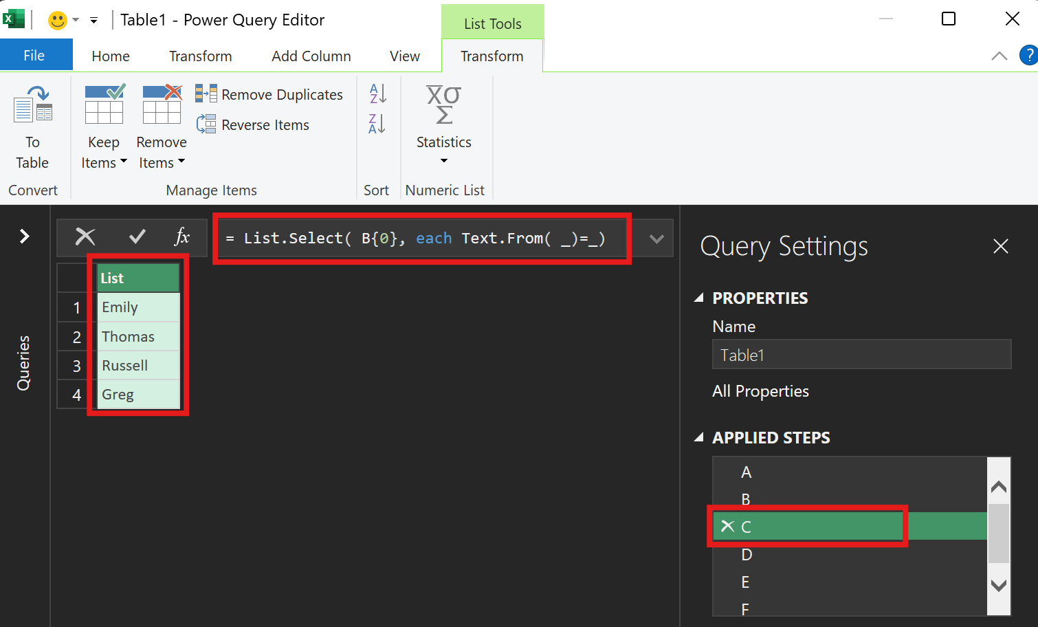
Step C output is below. All four names are extracted! Now we understand step B’s purpose. Step C uses list function List.Select to extract text items from the first nested list in step B.

We now know WHAT step C did but HOW did it do it? The formula bar displays this code:

= List.Select( B{0}, each Text.From(_)=_)

Remember: function syntax helps us unravel the mystery:

List.Select(list as list, selection as function) as list

list as list List.Select asks for a list. B{0} gives it the first embedded list from step B (M code is zero based meaning counting starts with 0 not 1).

each Text.From(_)=_) function Text.From converts each list item into a text. For each item, convert it to a text and compare =_ it to the original list value. If they’re both text then keep them! So, only original text values will be the same as values converted to text.

I played with the syntax and removed the comparison part at the end =_ Without this, all values become text and remain. A tricky piece of syntax!

It gives us a four item list of names (List.Select returns a list).

Step D

At a high level, step D says: give me the other stuff in the first nested list (NOT the four text names) and convert it to number.

= List.Transform( List.Difference( B{0}, C ),Number.From)

Explore the syntax seen above/below.

List.Transform(list as list, transform as function) as list

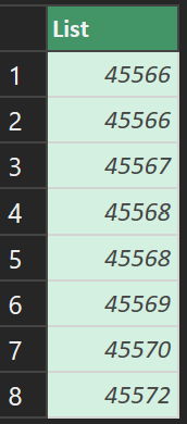
Step A reminds us the other stuff is eight date values (aka numbers):

Step E

Yes, the M code in step E is challenging (get coffee) but we can do it!

 E = List.Transform( 
       List.Split( 
          List.Transform({0..List.Count(D)-1}, each D{_}+List.RemoveNulls( B{1}{_}),
          2
       )
       ,(x)=> (x{1}-x{0})*24
     )

We’ll break it into three parts:

Step E inner part

List.Transform({0..List.Count(D)-1}, each D{_}+List.RemoveNulls(B{1}{_})

List.Transform wants a list then an action on the list then return a new list

List.Transform(list as list, transform as function) as list

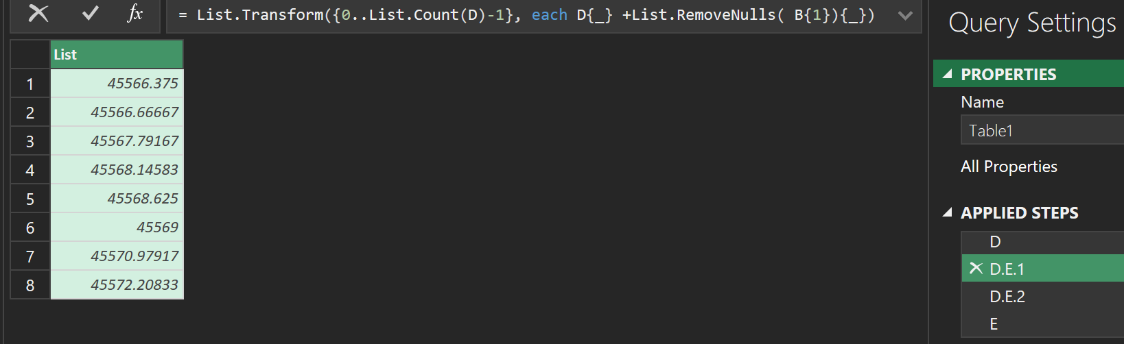
I wanted to see what it produced so I created step D.E.1:

Integer values (e.g. 45566) are dates. It adds time portion (day fraction between 0 and 1) to the integer! Now I know WHAT it creates but HOW?

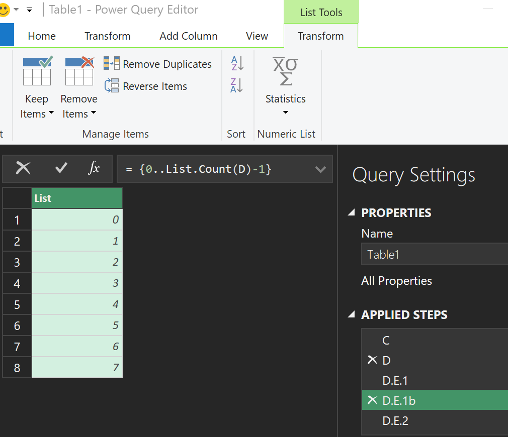
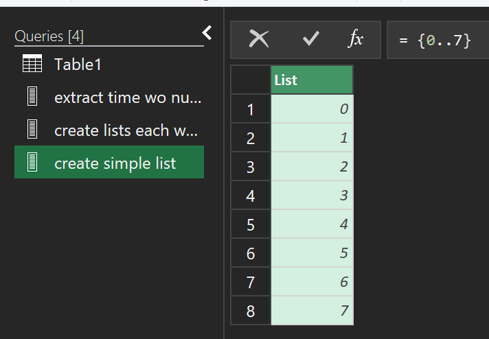
The list (inside List.Transform) part below creates a list from 0 to 7:

{0..List.Count(D)-1}

Below, ={0..7} creates list, always 0 to 7 Above, it’s dynamic via count function ={0..List.Count(D)-1}

This is perhaps the only part that I don’t 100% understand…but I think of it as creating eight rows so we can add eight date (integers) and time (decimals) values together.

Now, let’s see exactly what transform as function does:

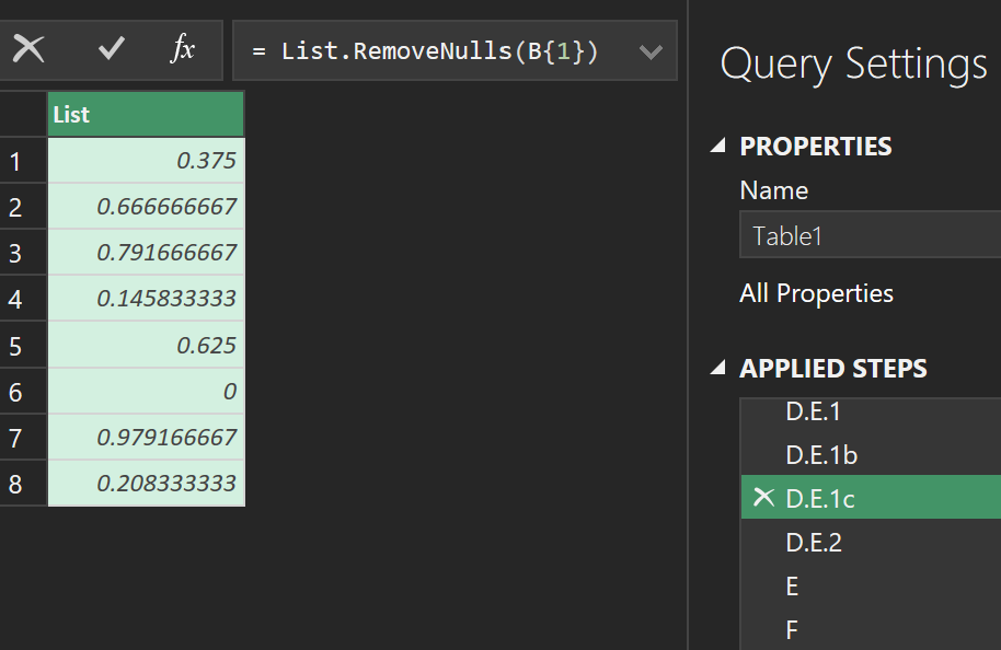
each D{_}+List.RemoveNulls( B{1}{_})

Key: we’ve been dealing with the first nested list from step B (dates). Now, Kris is extracting time values from the second nested list in step B. Function List.RemoveNulls removes the nulls.

I created another mini query to see this isolated part:

Step E middle part

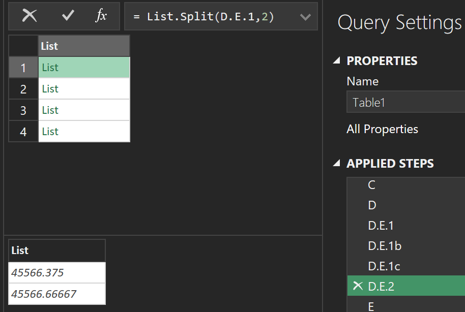
=List.Split(D.E.1,2)

List.Split wants a list then an action on the list then return a new list

List.Split(list as list, pageSize as number) as list

pageSize as number is 2 (two per nested list). To see it, I created this:

It’s easy to forget why we’re doing all this. Remember: per person, subtract start date time from end date time to create time duration!

List.Split creates four nested lists, one per person, with start date time and end date time inside each one. Above, I selected the first nested list so we can see it’s two values (bottom left).

Step E outer part

Each end date time – start date time. Multiply that amount by 24:

List.Transform wants a list then an action on the list then return a new list
List.Transform(list as list, transform as function) as list
(x)=> (x{1}-x{0})*24

What does (x)=> do? It says: let’s create a function called x, subtract the first nested item (start date time) from the second nested item (end date time), multiply that by 24.

I recommend Mike Girvin’s book to learn Power Query function syntax (and P.Q. in general):

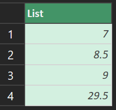
Step E’s final result is:

Step F

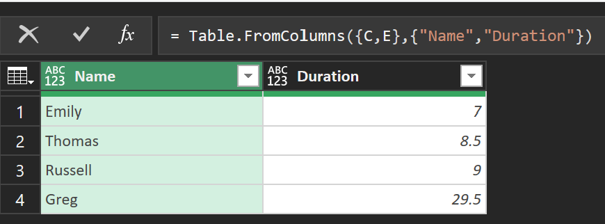
Table.FromColumns puts the steps together for the final answer.

=Table.FromColumns({C,E},{"Name","Duration"})
Table.FromColumns(lists as list, optional columns as any) as table

After a lot of List functions Kris uses a Table function!

Recap

  • as an advanced user, Kris did a lot of work in step E by combining functions
  • also, Kris named his steps in a sequential manner (A, B, C, etc.) because that’s all he needed
  • Kris can read M code like a sentence! I’m not there yet so I did the following:
    • wrote new queries to see exactly what data a particular part created
    • studied Microsoft’s M function syntax
    • horizontally aligned M code to make it easier to read
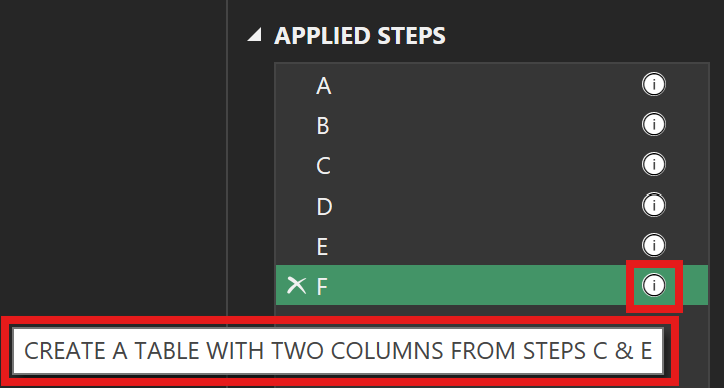
    • added comments viewable in advanced editor and in Applied Steps (hover over “i”)

When initially auditing Kris’ M code, I sketched it out to help understand it:

I added comments, indentation, and carriage returns to Kris’ code:

let

//CONNECT TO TABLE1
 A = Excel.CurrentWorkbook(){[Name="Table1"]}[Content],

//EACH COLUMN BECOMES A LIST ITEM
 B = Table.ToColumns(A),
 
//SELECT FIRST LIST AND EXTRACT TEXT VALUES 
 C = List.Select(B{0}, each Text.From(_)=_),
 
//EXTRACT DATE VALUES AND CONVERT TO NUMBER 
 D = List.Transform( List.Difference(B{0},C), Number.From),

//CALCULATE DURATION BETWEEN EACH PERSON'S DATE/TIME VALUES 
 E = List.Transform( 
                    List.Split( 
                               List.Transform({0..List.Count(D)-1}, each D{_}                                               
                               +List.RemoveNulls( B{1}){_}),
                               2
                    )
                    ,(x)=> (x{1}-x{0})*24
     ),

//CREATE A TABLE WITH TWO COLUMNS FROM STEPS C & E
 F = Table.FromColumns({C,E},{"Name","Duration"})

in
 F

After reviewing all the pieces, is the M code easier to read now? I hope so.

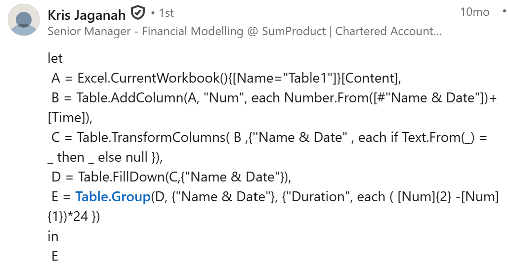
Here’s another Power Query solution by Kris for the same challenge!

let
 A = Excel.CurrentWorkbook(){[Name="Table1"]}[Content],
 B = Table.AddColumn(A, "Num", each Number.From([#"Name & Date"])+[Time]),
 C = Table.TransformColumns( B ,{"Name & Date" , each if Text.From(_) = _ then _ else null }),
 D = Table.FillDown(C,{"Name & Date"}),
 E = Table.Group(D, {"Name & Date"}, {"Duration", each ( [Num]{2} -[Num]{1})*24 })
in
 E

About Me

My name is Kevin Lehrbass. I’m a data analyst. I can *think* in Excel formulas easily. I’m training my brain more and more to *think* in M code and DAX…while also reviewing SQL and VBA!

Away from data, my other hobbies include: learning Spanish, playing chess, and drawing.